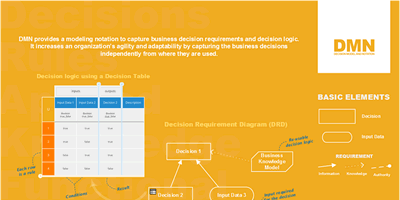
Bruce Silver's blog post - FEEL Operators Explained
Bruce Silver
Blog

FEEL Operators Explained

By Bruce Silver

Read Time: 5 Minutes

Although DMN’s expression language FEEL was designed to be business-friendly, it remains intimidating to many. That has led to the oft-heard charge that “DMN is too hard for business users”. That’s not true, at least for those willing to learn how to use it. Although the Microsoft Excel Formula language is actually less business-friendly than FEEL, somehow you never hear that “Excel is too hard for business users.”

One key reason why FEEL is more business-friendly than the Excel Formula language, which they now call Power FX, is its operators. FEEL has many, and Power FX has very few. In this post we’ll discuss what operators are, how they simplify the expression syntax, and how DMN boxed expressions make some FEEL operators more easily understood by business users.

It bears repeating that an expression language is not the same as a programming language. A programming language has statements. It defines variables, calculates and assigns their values. You could call DMN as a whole a programming language, but the expression language FEEL does not define variables or assign their values. Those things done graphically, in diagrams and tables – the DRD and boxed expressions. FEEL expressions are simply formulas that calculate values: data values in, data values out.

Functions and Operators

Those formulas are based on two primary constructs: functions and operators.

The logic of a function is specified in the function definition in terms of inputs called parameters. The same logic can be reused simply by invoking the function with different parameter values, called arguments. The syntax of function invocation – both in FEEL and Excel Formulas – is the function name immediately followed by parentheses enclosing a comma-separated list of arguments. FEEL provides a long list of built-in functions, meaning the function names and their parameters are defined by the language itself. Excel Formulas do the same. In addition, DMN allows modelers to create custom functions in the form of Business Knowledge Models (BKMs) and decision services, something Excel does not allow without programming.

Operators are based on reserved words and symbols in the expression with meaning defined by the expression language itself. There are no user-defined operators. They do not use the syntax of a name followed by parentheses enclosing a list of arguments. As a consequence, the syntax of an expression using operators is usually shorter, simpler, and easier to understand than an expression using functions.

You can see this from a few examples in FEEL where you could use either a function or an operator. One is simple addition. Compare the syntax of the expression adding variables a and b using the sum() function

sum(a, b)

with its equivalent using the addition operator +:

a + b

The FEEL function list contains() and the in operator do the same thing, test containment of a value in a list. Compare

list contains(myList, "abc")

with

"abc" in myList

Both FEEL and Excel support the basic arithmetic operators like +, -, *, and /, comparison operators like =, >, or <=, and string concatenation. But those are essentially the only operators provided by Excel, whereas FEEL provides several more. It is with these more complex operators that FEEL’s business-friendliness advantage stands out.

if..then..else

Let’s start with the conditional operator, if..then..else. These keywords comprise an operator in FEEL, where Excel can use only functions. Compare the FEEL expression

if Credit Score = "High" and Affordability = "OK" then "Approved" else "Disapproved"

with Excel’s function-based equivalent:

IF(AND(Credit Score = "High", Affordability = "OK"), "Approved", "Disapproved")

The length is about the same but the FEEL is more human-readable. Of course, the Excel expression assumes you have assigned a variable name to the cells – something no one ever does. So you would be more likely to see something like this:

IF(AND(B3 = "High", C3 = "OK"), "Approved", "Disapproved")

That is a trivial example. A more realistic if..then..else might be

if Credit Score = "High" and Affordability = "OK" then "Approved"
        else if Credit Score = "High" and Affordability = "Marginal" then "Referred"
        else "Disapproved"

That’s longer but still human-readable. Compare that with the Excel formula:

IF(AND(Credit Score = "High", Affordability= "OK"), "Approved", IF(AND(Credit Score = "High",
         Affordability = "Marginal"), "Referred", "Disapproved"))

Even though the FEEL syntax is fairly straightforward, DMN includes a conditional boxed expression that enters the if, then, and else expressions in separate cells, in theory making the operator friendlier for some users and less like code. Using that boxed expression, the logic above looks like this:

Filter

The FEEL filter operator is square brackets enclosing either a Boolean or integer expression, immediately following a list. When the enclosed expression is a Boolean, the filter selects items from the list for which the expression is true. When the enclosed expression evaluates to positive integer n, the filter selects the nth item in the list. (With negative integer n, it selects the nth item counting backward from the end.) In practice, the list you are filtering is usually a table, a list of rows representing table records, and the Boolean expression references columns of that table. I wrote about this last month in the context of lookup tables in DMN. As we saw then, if variable Bankrates is a table of available mortgage loan products like the one below,

then the filter

Bankrates[lenderName = "Citibank"]

selects the Citibank record from this table. Actually, a Boolean filter always returns a list, even if it contains just one item, so to extract the record from that list we need to append a second integer filter [1]. So the correct expression is

Bankrates[lenderName = "Citibank"][1]

Excel Formulas do not include a filter operator, but again use a function: FILTER(table, condition, else value). So if we had assigned cells A2:D11 to the name Bankrates and the column A2:A11 to the name lenderName, the equivalent Excel Formula would be

FILTER(Bankrates, lenderName = "Citibank", "")

but would more likely be entered as

FILTER(A2:D11, A2:A11 = "Citibank", "")

FEEL’s advantage becomes even more apparent with multiple query criteria. For example, the list of zero points/zero fees loan products in FEEL is

Bankrates[pointsPct = 0 and fees = 0]

whereas in Excel you would have

FILTER(A2:D11, (C2:C11=0)*(D2:D11=0), "")

There is no question here that FEEL is more business-friendly.

Iteration

The for..in..return operator iterates over an input list and returns an output list. It means for each item in the input list, to which we assign a dummy range variable name, calculate the value of the return expression:

for <range variable> in <input list> return <return expression, based on range variable>

It doesn’t matter what you name the range variable, also called the iterator, as long as it does not conflict with a real variable name in the model. I usually just use something generic like x, but naming the range variable to suggest the list item makes the expression more understandable. In the most common form of iteration, the input list is some expression that represents a list or table, and the range variable is an item in that list or row in that table.

For example, suppose we want to process the Bankrates table above and create a new table Payments by Lender with columns Lender Name and Monthly Payment, using a requested loan amount of $400,000. And suppose we have a BKM Lender Payment, with parameters Loan Product and Requested Amount, that creates one row of the new table, a structure with components Lender Name and Monthly Payment. We will iterate a call to this BKM over the rows of Bankrates using the for..in..return operator. Each iteration will create one row of Payments by Lender, so at the end we will have a complete table.

The literal expression for Payments by Lender is

for product in Bankrates return Lender Payment(product, Requested Amount)

Here product is the range variable, meaning one row of Bankrates, a structure with four components as we saw earlier. Bankrates is the input list that we iterate over. The BKM Lender Payment is the return expression.Beginners are sometimes intimidated by this literal expression, so, as with if..then..else, DMN provides an iterator boxed expression that enters the for, in, and return expressions in separate cells.

The BKM Lender Payment uses a context boxed expression with no final result box to create each row of the table. The context entry Monthly Payment invokes another BKM, Loan Amortization Formula, which calculates the value based on the adjusted loan amount, the interest rate, and fees.

Excel Formulas do not include an iteration function. Power FX’s FORALL function provides iteration, but it is not available in Excel. To iterate an expression in Excel you are expected to fill down in the spreadsheet.

The FEEL operators some..in..satisfies and every..in..satisfies represent another type of iteration. The range variable and input list are the same as with for..in..return. But in these expressions the satisfies clause is a Boolean expression, and the iteration operator returns not a list but a simple Boolean value. The one with some returns true if any iteration returns true, and the one with every returns true only if all iterations return true.

For example, again using Bankrates,

some product in Bankrates satisfies product.pointsPct = 0 and product.fees = 0

returns true, while

every product in Bankrates satisfies product.pointsPct = 0 and product.fees = 0

returns false. The iterator boxed expression works with this operator as well.

The bottom line is this: FEEL operators are key to its combination of expressive power and business-friendliness, surpassing that of Microsoft Excel Formulas. Modelers should not be intimidated by them. For detailed instruction and practice in using these and other DMN constructs, check out my DMN Method and Style training. You get 60-day use of Trisotech Decision Modeler and post-class certification at no additional cost.

Follow Bruce Silver on Method & Style.

Blog Articles

Bruce Silver

View all

All Blog Articles

Read our experts’ blog

View all

Bruce Silver's blog post - Lookup Tables in DMN
Bruce Silver
Blog

Lookup Tables in DMN

By Bruce Silver

Read Time: 5 Minutes

Lookup tables are a common logic pattern in decision models. To model them, I have found that beginners naturally gravitate to decision tables, being the most familiar type of value expression. But decision tables are almost never the right way to go. One basic reason is that we generally want to be able to modify the table data without creating a new version of the decision model, and with decision tables you cannot do that. Another reason is that decision tables must be keyed in by hand, whereas normal data tables can be uploaded from Excel, stored in a cloud datastore, or submitted programmatically as JSON or XML.

The best way to model a lookup table is a filter expression on a FEEL data table. There are several ways to model the data table – as submitted input data, a cloud datastore, a zero-input decision, or a calculated decision. Each way has its advantages in certain circumstances. In this post we’ll look at all the possibilities.

As an example, suppose we have a table of available 30-year fixed rate home mortgage products, differing in the interest rate, points (an addition to the requested amount as a way to “buy down” the interest rate), and fixed fees. You can find this data on the web, and the rates change daily. In our decision service, we want to allow users to find the current rate for a particular lender, and in addition find the monthly payment for that lender, which depends on the requested loan amount. Finding the lender’s current rate is a basic lookup of unmodified external data. Finding the monthly payment using that lender requires additional calculation. Let’s look at some different ways to model this.

We can start with a table of lenders and rates, either keyed in or captured by web scraping. In Excel it looks like this:

When we import the Excel table into DMN, we get a FEEL table of type Collection of tBankrate, shown here:

Each row of the table, type tBankrate, has components matching the table columns. Designating a type as tPercent simply reminds us that the number value represents a percent, not a decimal.

Here is one way to model this, using a lookup of the unmodified external data, and then applying additional logic to the returned value.

We define the input data Bankrates as type Collection of tBankrate and lookup my rate – the one that applies to input data my lender. The lookup decision my rate uses a filter expression. A data table filter typically has the format

<table>[<Boolean expression of table columns>]

in which the filter, enclosed in square brackets, contains a Boolean expression. Here the table is Bankrates and the Boolean expression is lenderName = my lender. In other words, select the row for which column lenderName matches the input data my lender.

A filter always returns a list, even if it contains just one item. To extract the item from this list, we use a second form of a filter, in which the square brackets enclose an integer:

<list>[<integer expression>]

In this case, we know our data table just has a single entry for each lender, so we can extract the selected row from the first filter by appending the filter [1]. The result is no longer a list but a single row in the table, type tBankrate.

The decision my payment uses a BKM holding the Loan Amortization Formula, a complicated arithmetic expression involving the loan principal (p), interest rate (r), and number of payments (n), in this case 360.

Decision my payment invokes this BKM using the lookup result my rate. Input data loan amount is just the borrower’s requested amount, but the loan principal used in Loan Amortization Formula (parameter p) also includes the lender’s points and fees. Since pointsPct and ratePct in our data table are expressed as percent, we need to divide by 100 to get their decimal value used in the BKM formula.

When we run it with my lender “Citibank” and loan amount $400,000, we get the result shown here.

That is one way to do it. Another way is to enrich the external data table with additional columns, such as the monthly payment for a given loan amount, and then perform the lookup on this enriched data table. In that case the data table is a decision, not input data.

Here the enriched table Payments by Bank has an additional column, payment, based on the input data loan amount. Adding a column to a table involves iteration over the table rows, each iteration generating a new row including the additional column. In the past I have typically used a context BKM with no final result box to generate the each new row. But actually it is simpler to use a literal expression with the context put() function, as no BKM is required to generate the row, although we still need the Loan Amortization Formula. (Simpler for me, but the resulting literal expression is admittedly daunting, so I’ll show you an alternative boxed expression that breaks it into simpler pieces.)

context put(), with parameters context, keys, and value, appends components (named by keys) to a an existing structure (context), and assigns their value. If keys includes an existing component of context, value overwrites the previous value. Here keys is the new column name “payment”, and value is calculated using the BKM Loan Amortization Formula. So, as a single literal expression, Payments by Bank looks like this:

Here we used literal invocation of the BKM instead of boxed invocation, and we applied the decimal() function to round the result.

Alternatively, we can use the iterator boxed expression instead of the literal for..in..return operator and invocation boxed expressions for the built-in functions decimal() and context put() as well as the BKM. With FEEL built-in functions you usually use literal invocation but you can use boxed invocation just as well.

Now my payment is a simple lookup of the enriched data table Payments by Bank, appending the [1] filter to extract the row and then .payment to extract the payment value for that row.

When we run it, we get the same result for Citibank, loan amount $400,000:

The enriched data table now allows more flexibility in the queries. For example, instead of finding the payment for a particular lender, you could use a filter expression to find the loan product(s) with the lowest monthly payment:

Payments by Bank[payment=min(Payments by Bank.payment)]

which returns a single record, AimLoan. Of course, you can also use the filter query to select a number of records meeting your criteria. For example,

Payments by Bank[payment < 2650]

will return records for AimLoan, AnnieMac, Commonwealth, and Consumer Direct.

Payments by Bank[pointsPct=0 and fees=0]

will return records for zero-points/zero-fee loan products: Aurora Financial, Commonwealth, and eLend.

Both of these methods require submitting the data table Bankrates at time of execution. Our example table was small, but in real projects the data table could be quite large, with thousands of rows. This is more of a problem for testing in the modeling environment, since with the deployed service the data is submitted programmatically as JSON or XML. But to simplify testing, there are a couple ways you can avoid having to input the data table each time.

You can make the data table a zero-input decision using a Relation boxed expression. On the Trisotech platform, you can populate the Relation with upload from Excel. To run this you merely need to enter values for my lender and loan amount. You can do this in production as well, but remember, with a zero-input decision you cannot change the Bankrates values without versioning the model.

Alternatively, you can leave Bankrates as input data but bind it to a cloud datastore. Via an admin interface you can upload the Excel table into the datastore, where it is persisted as a FEEL table. So in the decision model, you don’t need to submit the table data on execution, and you can periodically update the Bankrates values without versioning the model. Icons on the input data in the DRD indicate its values are locked to the datastore.

Lookup tables using filter expressions are a basic pattern you will use all the time in DMN. For more information on using DMN in your organization’s decision automation projects, check out my DMN Method and Style training or my new book, DMN Method and Style 3rd edition, with DMN Cookbook.

Follow Bruce Silver on Method & Style.

Blog Articles

Bruce Silver

View all

All Blog Articles

Read our experts’ blog

View all

Dr. John Svirbely's blog post - Going from Zero to Success using BPM+ for Healthcare. 
                Part I: Learning Modeling and Notation Tools
Dr. John Svirbely, MD
Blog

Going from Zero to Success using BPM+ for Healthcare.

Part I:
Learning Modeling and Notation Tools

By Dr. John Svirbely, MD

Read Time: 3 Minutes

Welcome to the first installment of this informative three-part series providing an overview of the resources and the success factors required to develop innovative, interoperable healthcare workflow and decision applications using the BPM+ family of open standards. This series will unravel the complexities and necessities for achieving success with your first clinical guideline automation project. Part I focuses on how long it will take you to reach cruising speed for creating BPM+ visual models.

When starting something new, people often ask some common questions. One is how long will it take to learn the new skills required. This impacts how long it will take to complete a project and therefore costs. Learning something new can also be somewhat painful when we are set in our old ways.

Asking such questions is important, since there is often a disconnect between what is promoted online and the reality. I can give my perspective based on using the Trisotech tools for several years, starting essentially from scratch.

How long does it take to learn?

The simple answer – it depends. A small project can be tackled by a single person quite rapidly. That is how I got started. Major projects using these tools should be approached as team projects rather than something an individual can do. Sure, there are people who can master a wide range of skills, but in general most people are better at some things than others. Focusing on a few things is more productive than trying to do everything. A person can become familiar with the range of tools, but they need to realize that they may only be able to unlock a part of what is needed to automate a clinical guideline.

The roles that need to be filled to automate a clinical guideline with BPM+ include:

1 subject matter expert (SME)

2 medical informaticist

3 visual model builder

4 hospital programmer/system integrator

5 project manager

6 and of course, tester

A team may need to be composed of various people who bring a range of skills and fill various roles. A larger project may need more than one person in some of these roles.

The amount of time needed to bring a subject matter expert (SME) up to speed is relatively short. Most modeling diagrams can be understood and followed after a few days. I personally use a tool called the Knowledge Entity Modeler (KEM) to document domain knowledge; this allows specification of term definitions, clinical coding, concepts maps and rule definitions. The KEM is based on the SVBR standard, but its visual interface makes everything simple to grasp. Other comparable visual tools are available. The time spent is quickly compensated for by greater efficiency in knowledge transfer.

The medical informaticist has a number of essential tasks such as controlling terminology, standardizing data, and assigning code terms. The person must understand the nuances of how clinical data is acquired including FHIR. These services cannot be underestimated since failures here can cause many problems later as the number of models increase or as models from different sources are installed.

The model builder uses the various visual modelling languages (DMN, BPMN, CMMN) according to the processes and decisions specified by the SME. These tools can be learned quickly to some extent, but there are nuances that may take years to master. While some people can teach themselves from books or videos, the benefits of taking a formal course vastly outweigh the cost and time spent. Trsiotech offers eLearning modules that you can learn from at your own pace.

When building models, there is a world of difference between a notional model and one that is automatable. Notional models are good for knowledge capture and transfer. A notional model may look good on paper only to fail when one tries to automate it. The reasons for this will be discussed in Part 3 of this blog series.

The hospital programmer or system integrator is the person who connects the models with the local EHR or FHIR server so that the necessary data is available. Tools based on CDS Hooks or SMART on FHIR can integrate the models into the clinical workflow so that they can be used by clinicians. This person may not need to learn the modeling tools to perform these tasks.

The job of the project manager is primarily standard project management. Some knowledge of the technologies is helpful for understanding the problems that arise. This person’s main task is to orchestrate the entire project so that it keeps focused and on schedule. In addition, the person keeps chief administrators up to date and tries to get adequate resources.

The final player is the tester. Testing prior to release is best done independently of other team members to maintain objectivity. There is potential for liability with any medical software, and these tools are no exception. This person also oversees other quality measures such as bug reports and complaints. Knowing the modeling languages is helpful but understanding how to test software is more important.

My journey

I am a retired pathologist and not a programmer. While having used computers for many years, my career was spent working in community hospitals. When I first encountered the BPM+ standards, it took several months and a lot of prodding before I was convinced to take formal training. I have never regretted that decision and wish that I had taken training sooner.

I started with DMN. On-line training takes about a month. After an additional month I had enough familiarity to become productive. In the following 12 months I was able to generate over 1,000 DMN models while doing many other things. It was not uncommon to generate 4 models in one day.

I learned BPMN next. Training online again took a month. This takes a bit longer to learn because it requires an appreciation of how to design a process so that it executes optimally. Initially a model would take me 2-3 days to complete, but later this dropped to less than a day. Complex models can take longer, especially when multiple people need to be orchestrated and exception handling is introduced.

CMMN, although offering great promise for healthcare, is a tough nut to crack. Training is harder to arrange, and few vendors offer automatable versions. This standard is better saved until the other standards have been mastered.

What are the barriers?

Most of the difficulties that I have encountered have not been related to using the standards. They usually arise from organizational or operational issues. Some common barriers that I have encountered include:

1 lack of clear objectives, or objectives that constantly change.

2 lack of commitment from management, with insufficient resources.

3 unrealistic expectations.

4 rushing into models before adequate preparations are made.

If these can be avoided, then most projects can be completed in a satisfactory manner. How long it takes to implement a clinical guideline will be discussed in the next blog.

Blog Articles

John Svirbely

View all

All Blog Articles

Read our experts’ blog

View all

Bruce Silver's blog post - DMN 101
Bruce Silver
Blog

DMN 101

By Bruce Silver

Read Time: 4 Minutes

Most of my past posts about DMN have assumed that the reader knows what it is and may be using it already. But there is undoubtedly a larger group of readers who have heard about it but don’t really understand what it’s all about. And possibly an equally large group that have heard about it from detractors and have some misconceptions. So in this post I will try to explain what it is and how it works.

DMN, which stands for Decision Model and Notation, is a model-based language for business decision logic. Furthermore, it is a vendor-neutral standard maintained by the Object Management Group (OMG), the organization behind BPMN, CMMN, and other standards. As with OMG’s other business modeling standards, “model” means the names, meaning, and execution behavior of each language element are formally defined in a UML metamodel, and “notation” means that a significant portion of the language is defined graphically, in diagrams and tables using specific shapes and symbols linked to model elements. In other words, the logic of a business decision, business process, or case is defined by diagrams having a precise meaning, independent of the tool that created them. The main reason for defining the logic graphically is to engage non-programmers, aka business people, in their creation and maintenance.

DMN models the logic of operational decisions, those made many times a day following the same explicit rules. Examples include approval of a loan, validation of submitted data, or determining the next best action in a customer service request. These decisions typically depend on multiple factors, and the logic is frequently complex. The most familiar form of DMN logic is the decision table. All DMN tools support decision tables, and that’s because business people understand them readily with zero training. Consider the decision table below, which estimates the likelihood of qualifying for a home mortgage:

Qualifying for a home mortgage depends primarily on three factors: the borrower’s Credit Score, a measure of creditworthiness; the Loan-to-Value ratio, dividing the loan amount by the property appraised value, expressed as a percent; and the borrower’s Debt-to-Income ratio, dividing monthly housing costs plus other loan payments by monthly income, expressed as a percent. Those three decision table inputs are represented by the columns to the left of the double line. The decision table output, here named Loan Prequalification, with possible values “Likely approved”, “Possibly approved”, “Likely disapproved”, or “Disapproved”, is the column to the right of the double line. Below the column name is its datatype, including allowed values. Each numbered row of the table is a decision rule. Cells in the input columns are conditions on the input, and if all input conditions for a rule evaluate to true, the rule is said to match and the value in the output column is selected as the decision table output value.

A hyphen in an input column means the input is not used in the rule; the condition is true by default. So the first rule says, if Credit Score is less than 620, Loan Prequalification is “Disapproved”. Numeric ranges are shown as values separated by two dots, all enclosed in parentheses or square brackets. Parenthesis means exclude the endpoint in the range; square bracket means include it. So rule 4 says, if Credit Score is greater than or equal to 620 and less than 660, and LTV Pct is greater than 75 and less than or equal to 80, and DTI Pct is greater than 36 and less than or equal to 45, then Loan Prequalification is “Likely disapproved”. Once you get the numeric range notation, the meaning of the decision table is clear, and this is a key reason why DMN is considered business-friendly.

But if you think harder about it, you see that while Credit Score might be a known input value, LTV Pct and DTI Pct are not. They are derived values. They are calculated from known input values such as the loan amount, appraised property value, monthly income, housing expense including mortgage payment, tax, and insurance, and other loan payments. In DMN, those calculations are provided as supporting decisions to the top-level decision Loan Prequalification. Each calculation itself could be complex, based on other supporting decisions. This leads to DMN’s other universally supported feature, the Decision Requirements Diagram, or DRD. Below you see the DRD for Loan Prequalification. The ovals are input data, known input values, and the rectangles are decisions, or calculated values. The solid arrows pointing into a decision, called information requirements, define the inputs to the decision’s calculations, either input data or supporting decisions.

Like decision tables, DRDs are readily understood by business users, who can create them to outline the dependencies of the overall logic. In the view above, we show the datatype of each input data and decision in the DRD. Built-in datatypes include things like Text, Number, Boolean, and collections of those, but DMN also allows the modeler to create user-defined types representing constraints on the built-in types – such as the numeric range 300 to 850 for type tCreditScore – and structured types, specified as a hierarchy of components. For example, tLoan, describing the input data Loan, is the structure seen below:

Individual components of the structure are referenced using a dot notation. For example, the Loan Amount value is Loan.Amount.

A complete DRD, therefore, including datatypes for all supporting decisions down to input data, provides significant business value and can be created easily by subject matter experts. As a consequence, all DMN tools support DRDs. But by itself, the DRD and a top-level decision table is not enough to evaluate the decision. For that you need to provide the logic for the supporting decisions. And here there is some disagreement within the DMN community. Some tool vendors believe that DMN should be used only to provide model-based business requirements. Those requirements are then handed offto developers for completion of the decision logic using some other language, either a programming language like Java or a proprietary business rule language like IBM ODM. I call those tools DMN Lite, because fully implemented DMN allows subject matter experts to define the complete, fully executabledecision logic themselves, without programming.

Full DMN adds two key innovations to DRDs and decision tables: the expression language FEEL and standardized tabular formats called boxed expressions. Using boxed expressions and FEEL, real DMN tools let non-programmers create executable decision models, even when the logic is quite complex. So you can think of DMN as a Low-Code language for decision logic that is business-friendly, transparent, and executable.

In that language, the shapes in the DRD define variables (with assigned datatypes), with the shape labels defining the variable names. Defining variables by drawing the DRD explains an unusual feature of FEEL, which is that variable names may contain spaces and other punctuation not normally allowed by programming languages. The value expression of each individual decision is the calculation of that decision variable’s value based on the values of its inputs, or information requirements. It is the intention of FEEL and boxed expressions that subject matter experts who are not programmers can create the value expressions themselves.

FEEL is called an expression language, a formula language like Excel formulas, as opposed to a programming language. FEEL just provides a formula for calculating an output value based on a set of input values. It does not create the output and input variables; the DRD does that. Referring back to our DRD, let’s look at the value expression for LTV Pct, the Loan-to-Value ratio expressed as a percent. The FEEL expression looks like this:

It’s simple arithmetic. Anyone can understand it. This is the simplest boxed expression type, called a literal expression, just a FEEL formula in a box, with the decision name and datatype in a tab at the top. Decision table is another boxed expression type, and there are a few more. Each boxed expression type has a distinct tabular format and meaning, and cells in those tables are FEEL expressions. In similar fashion, here is the literal expression for DTI Pct:

The tricky one is Mortgage Payment. It’s also just arithmetic, based on the components of Loan. But the formula is hard to remember, even harder to derive. And it’s one that in lending is used all the time. For that, the calculation is delegated to a bit of reusable decision logic called a Business Knowledge Model, or BKM. In the DRD, it’s represented as a box with two clipped corners, with a dashed arrow connecting it to a decision. A BKM does not have incoming solid arrows, or information requirements. Instead, its inputs are parameters defined by the BKM itself. BKMs provide two benefits: One, they allow the decision modeler to delegate the calculation to another user, possibly with more technical or subject matter knowledge, and use it in the model. Two, it allows that calculation to be defined once and reused in multiple decision models. The dashed arrow, called a knowledge requirement, signifies that the decision at the head of the arrow passes parameter values to the BKM, which then returns its output value to the decision. We say the decision invokes the BKM, like calling an api. The BKM parameter names are usually different from the variable names in the decision that invokes them. Instead, the invocation is a data mapping.

Here I have that BKM previously saved in my model repository under the name Loan Amortization Formula. On the Trisotech platform, I can simply drag it out onto the DRD and replace the BKM Payment Calculation with it. The BKM definition is shown below, along with an explanation of its use from the BKM Description panel. It has three parameters – p, r, and n, representing the loan amount, rate, and number of payments over the term – shown in parentheses above the value expression. The value expression is again a FEEL literal expression. It can only reference the parameters. The formula is just arithmetic – the ** symbol is FEEL’s exponentiation operator – but as you see, it’s complicated.

The decision Mortgage Payment invokes the BKM by supplying values to the parameters p, r, and n, mappings from the decision’s own input, Loan. We could use a literal expression for this, but DMN provides another boxed expression type called Invocation, which is more business-friendly:

In a boxed Invocation, the name of the invoked BKM is below the tab, and below that is a two-column table, with the BKM parameter names in the first column and their value expressions in the second column. Note that because Loan.Rate Pct is expressed as a percent, we need to divide its value by 100 to get r, which is a decimal value, not a percent.

At this point, our decision model is complete. But we need to test it! I can’t emphasize enough how important it is to ensure that your decision logic runs without error and returns the expected result. So let’s do that now, using the input data values below:

Here Loan Prequalification returns “Possibly approved”, and the supporting decision values look reasonable. We can look at the decision table and see that rule 8 is the one that matches.

So you see, DMN is something subject matter experts who are not programmers can use in their daily work. Of course, FEEL expressions can do more than arithmetic, and like Excel formulas, the language includes a long list of built-in functions that operate on text, numbers, dates and times, data structures, and lists. I’ve discussed much of that in my previous posts on DMN. But learning to use the full power of FEEL and boxed expressions – which you will need in real-world decision modeling projects – generally requires training. Our DMN Method and Style training gives you all that, including 60-day use of Trisotech Decision Modeler, lots of hands-on exercises, quizzes to test your understanding, and post-class certification in which you need to create a decision model containing certain required elements. It’s actually in perfecting that certification model that the finer points of the training finally sink in. And you need that full 60 days to really understand DMN’s capabilities.

DMN lets you accelerate time-to-value by engaging subject matter experts directly in the solution. If you want to see if DMN is right for you, check out the DMN training.

Follow Bruce Silver on Method & Style.

Blog Articles

Bruce Silver

View all

All Blog Articles

Read our experts’ blog

View all

Bruce Silver's blog post - More On DMN Validation
Bruce Silver
Blog

More On DMN Validation

By Bruce Silver

Read Time: 5 Minutes

This month we return to a topic I’ve written about twice before, data validation in DMN models. This post, in which I will describe a third method, is hopefully the last word.

Beginning decision modelers generally assume that the input data supplied at execution time is complete and valid. But that is not always the case, and when input data is missing or invalid the invoked decision service returns either an error or an incorrect result. When the service returns an error result, typically processing stops at the first one and the error message generated deep within the runtime is too cryptic to be helpful to the modeler. So it is important to precede the main decision logic with a data validation service, either as part of the same decision model or a separate one. It should report all validation errors, not stop at the first one, and should allow more helpful, modeler-defined error messages. There is more than one way to do that, and it turns out that the design of that validation service depends on details of the use case.

The first method, which I wrote about in April 2021, uses a Collect decision table with generalized unary tests to find null or invalid input values, as you see below. When I introduced my DMN training, I thought this was the best way to do it, but it’s really ideal only for the simple models I was using in that training. That is because the method assumes that values used in the logic are easily extracted from the input data, and that the rule logic is readily expressed in a generalized unary test. Moreover, because an error in the decision table will usually fail without indicating which rule had the problem, the method assumes a modest number of rules with fairly simple validation expressions. As a consequence, this method is best used when:

The second method, which I wrote about in March 2023, takes advantage of enhanced type checking against the item definition, a new feature of DMN1.5. Unlike the first method, this one returns an error result when validation errors are present, but it returns all errors, not just the first one, each with a modeler-defined error message. Below you see the enhanced type definition, using generalized unary tests, and the modeler-defined error messages when testing in the Trisotech Decision Modeler. Those same error messages are returned in the fault message when executed as a decision service. On the Trisotech platform, this enhanced type checking can be either disabled, enabled only for input data, or enabled for input data and decisions.

This method of data validation is avoids many of the limitations of the first method, but cannot be used if you want the decision service to return a normal response, not a fault, when validation errors are present. Thus it is applicable when:

More recently I have been involved in a large data validation project in which neither of these methods are ideal. Here the input data is a massive data structure containing several hundred elements to be validated, and we want validation errors to generate a normal response, not a fault, with helpful error messages. Moreover, data values used in the rules are often buried deeply within the structure and many of them recurring, so simply extracting their values properly is non-trivial. Think of a tax return or loan application. And once you’ve extracted the needed data values, the validation rules themselves may be complex, depending on conditions of many other variables in the structure.

For these reasons, neither of the two methods described in my previous posts fit the bill here. Because an element’s validation rule can be a complex expression involving multiple elements, this rules out the type-checking method and is a problem as well for the Collect decision table. Decision tables also add the problem of testing. When you have many rules, some of them are going to be coded incorrectly the first time, and if a rule returns an error the whole decision table fails, so debugging is extremely difficult. Moreover, if a rule fails to return the expected result, you need to be able to determine whether it’s because you have incorrectly extracted the data element value or you have incorrectly defined the rule logic. Your validation method needs to separate those concerns.

This defines a new set of requirements:

The third method thus requires a more complex architecture, comprising:

While overkill for simple validation services, in complex validation scenarios this method has a number of distinct advantages over the other two:

Let’s walk through this third data validation method. We start with the Extraction service. The input data Complex Input has the structure shown here:

In this case there is only one non-repeating component, containing just two child elements, and one repeating component, also containing just two child elements. In the project I am working on, there are around 10 non-repeating components and 50 repeating components, many containing 10 or more child elements. So this model is much simpler than the one in my engagement.

The Extraction DRD has a separate branch for each non-repeating and each repeating component. Repeating element branches must iterate a BKM that extracts the individual elements for that instance.

The decisions ending in “Elements” extract all the variables referenced in the validation rules. These are not identical to the elements contained in Complex Input. For example, element A1 is just the value of the input data element A1, but element A1Other is either the input data element A2, if the value of A1 is “Other”, or null otherwise.

Repeating component branches must iterate a BKM that extracts the variable from a single instance of the branch.

In this case, we are extracting three variables – C1, AllCn, and Ctotal – although AllCn is just used in the calculation of Ctotal, not used in a rule. The goal of Extraction is just to obtain the values of variables used in the validation rules.

The ExtractAll service will be invoked by the Rules, and again the model has one branch for each non-repeating component and one for each repeating component. Encapsulating ExtractAll as a separate service is not necessary in a model this simple, but when there are dozens of branches it helps.

Let’s focus on Repeating Component Errors, which iterates a BKM that reports errors for a single instance of that branch.

In this example we have just two validation rules. One reports an error if element C1 is null, i.e. missing in the input. The other reports an error if element Ctotal is not greater than 0. The BKM here is a context, one context entry per rule, and all context entries have the same type, tRuleData, with the four components shown here. We could have added a fifth component containing the error message text, but here we assume that is looked up from a separate table based on the RuleID.

So the datatype tRepeatingComponentError is a context containing a context, and the decision Repeating Component Errors is a collection of a context containing a context. And to collect all the errors, we have one of these for each branch in the model.

That is an unwieldy format. We’d really like to collect the output for all the rules – with isError either true or false – in a single table. The decision ErrorTable provides that, using the little-known FEEL function get entries(). This function converts a context into a table of key-value pairs,and we want to apply it to the inner context, i.e. a single context entry of Repeating Component Error.

It might take a minute to wrap your head around this logic. Here fRow is a function definition – basically a BKM as a context entry – that converts the output of get entries() into a table row containing the key as a column. For non-repeating branches, we iterate over each error, calling get entries() on each one. This generates a table with one row per error and five columns. For repeating branches, we need to iterate over both the branches and for the errors in each branch, an iteration nested in another iteration. That creates a list of lists, so we need the flatten() function to make that a simple list, again one row per error (across all instances of the branch) and five columns. In the final result box, we just concatenate the tables to make one table for all errors in the model.

Here is the output of ErrorTable when run with the inputs below:

ErrorTable as shown here lists all the rules, whether an error or not. This is good for testing your logic. Once tested, you can easily filter this table to list only rules for which isError is true.

Bottom Line: Validating input data is always important in real-world decision services. We’ve now seen three different ways to do it, with different features and applicable in different use cases.

Follow Bruce Silver on Method & Style.

Blog Articles

Bruce Silver

View all

All Blog Articles

Read our experts’ blog

View all

Bruce Silver's blog post - Calendar Arithmetic in DMN
Bruce Silver
Blog

Calendar Arithmetic in DMN

By Bruce Silver

Read Time: 4 Minutes

Often in decision models you need to calculate a date or duration. For example, an application must be submitted within 90 days of some event, or a vaccine should not be administered within 120 days of a previous dose. DMN has powerful calendar arithmetic features. This post will illustrate how to use them.

ISO 8601 Format

The FEEL expressions for dates, times, and durations may look strange, but don’t blame DMN for that. They are based on the formats defined by ISO 8601, the international standard for dates and times in many computer languages. In FEEL expressions, dates and times can be specified by using a constructor function, e.g. date(), applied to a literal string value in ISO format, as seen below. For input and output data values, the constructor function is omitted.

A date is a 4-digit year, hyphen, 2-digit month, hyphen, 2-digit day. For example, to express May 3, 2017 as an input data value, just write 2015-05-03. But in a FEEL expression you must write date(2017-05-03).

Time is based on a 24-hour clock, no am/pm. The format is a 2-digit hour, 2-digit minute, 2-digit second, with optional fractional seconds after the decimal point. There is also an optional time offset field, representing the time zone expressed as an offset from UTC, what they used to call Greenwich Mean Time. For example, to specify 1:10 pm and 30 seconds Pacific Daylight Time, which is UTC 7 hours, you would enter 13:10:30-07:00 as an input data value, or time(13:10:30-07:00) in a FEEL expression. To specify the time as UTC, you can either use 00:00 as the time offset, or the letter Z, which stands for Zulu, which is the military symbol for UTC. DateTime values concatenate the date and time formats with a capital T separating them, as you see here. In a FEEL expression, you must use the proper constructor function with the ISO text string enclosed in quotes.

Date and Time Components

It is possible in FEEL to extract the year, month, or day component from a date, time, or dateTime using a dot followed by the component name: year, month, day, hour, minute, second, or time offset. For example, the expression date(“2017-05-03”).year returns the number 2017. All of these extractions return a number except for the time offset component, which returns not a number but a duration, with a format well discuss shortly.

DMN also provides an attribute, weekday not really a component but also extracted via dot notation returning an integer from 1 to 7, with 1 meaning Monday and 7 meaning Sunday.

Durations

The interval between two dates, times, or dateTimes defines a duration. DMN, like ISO, defines two kinds of duration: days and time duration, and years and months duration. Days and time duration is equivalent to the number of seconds in the duration. The ISO format is PdDThHmMsS, where the lower case d,h,m, and s are integers indicating the days, hours, minutes, and seconds in the duration. If any of them is zero, they are omitted along with the corresponding uppercase D, H, M, or S. And they are supposed to be normalized so that the sum of the component values is minimized.

For example a duration of 61 seconds could be written P0DT61S, but we can omit the 0D, and the normalized form is 1 minute 1 second, so the correct value is PT1M1S. In a FEEL expression, you need to enclose that in quotes and make it the argument of the duration constructor function: duration(“PT1M1S”).

Days and time duration is the one normally used in calendar arithmetic, but for long durations the alternative years and months duration is available, equivalent to the number of whole months included in the duration. The ISO format is PyYmM, where lower case y and m are again numbers representing number of years and months in the duration, and again the normalized form minimizes the sum of those component values. So a duration of 14 months would be written in normalized form as P1Y2M, and in FEEL, duration(P1Y2M). Since months contain varying numbers of days, the precise value of years and months duration is the number of months in between the start date and the end date, plus 1 if the day of the end month is greater than or equal to the day of the start month, or plus 0 otherwise.

As with dates and times, you can extract the components of a duration using a dot notation. For days and time duration, the components are days, hours, minutes, and seconds. For years and months duration, the components are years and months.

Arithmetic Expressions

The point of all this is to be able to do calendar arithmetic.

Lets start with addition of a duration.

A common use of calendar arithmetic is finding the difference between two dates or dateTimes.

You can multiply a duration times a number to get another duration of the same type, either days and time duration or years and months duration.

You can divide a duration by a number to get another duration of the same type.But the really useful one is dividing a duration by a duration, giving a number. For example, to find the number of seconds in a year, the expression duration(“P365D”)/duration(“PT1S”) returns the correct value, number 31536000. Note this is not the result returned by extracting the seconds component. The expression duration(P365D).seconds returns 0.

Example:
Refund Eligibility

Here is a simple example of calendar arithmetic from the DMN training. Given the purchase date and the timestamp of item return, determine the eligibility for a refund, based on simple rules.

The solution, using calendar arithmetic, is shown below:

Here we use a context in which the first context entry computes a days and time duration by subtracting the two dateTimes. The second context entry is a decision table that applies the rules. Note we can use durations like any other FEEL type in the decision table input entries.

Example:
Unix Timestamp

A second example comes from the Low-Code Business Automation training. It is common for databases and REST services to express dateTime values as a simple number. One common format used is the Unix timestamp, defined as the number of seconds since January 1, 1970, midnight UTC. To convert a Unix timestamp to a FEEL dateTime, you can use the BKM below:

The BKM multiplies the duration of one second by timestamp, a number, returning a days and time duration, and then adds that to the dateTime of January 1, 1970 midnight UTC, giving a dateTime. And you can perform the reverse mapping with the BKM below:

This time we subtract January 1, 1970 midnight UTC from the FEEL dateTime, giving a days and time duration, and then divide that by the duration one second, giving a number.

Calendar arithmetic is used all the time in both decision models and Low-Code business automation models. While the formats are unfamiliar at first, FEEL makes calendar arithmetic very easy. It’s all explained in the training. Both the DMN Method and Style course and the Low-Code Business Automation course provide 60-day use of the Trisotech platform and include post-class certification. Check out!

Follow Bruce Silver on Method & Style.

Blog Articles

Bruce Silver

View all

All Blog Articles

Read our experts’ blog

View all

What is FEEL?

FEEL (Friendly Enough Expression Language) is a powerful and flexible standard expression language developed by the OMG® (Object Management Group) as part of the Decision Model and Notation (DMN™) international standard.

Request a demo

Low-code/No-Code/Pro-Code

It is a valuable tool for modeling and managing decision logic in many domains, including healthcare, finance, insurance, and supply chain management. FEEL is designed specifically for decision modeling and execution and to be human-readable to business users, while still maintaining the expressive power needed for complex decision-making. Its simplicity, expressiveness, domain-agnostic functionality, strong typing, extensibility, and standardization make FEEL a valuable tool for representing and executing complex decision logic in a clear and efficient manner. Organizations using FEEL enjoy better collaboration, increased productivity, and more accurate decision-making.

What Are Expression Languages?

FEEL is a low-code expression language, but what is the difference between Expression Languages, Scripting Languages, and Programming Languages. They are all different types of languages used to write code, but they have distinct characteristics and uses.

Expression Languages

Expression languages are primarily designed for data manipulation and configuration purposes. They are focused on evaluating expressions rather than providing full-fledged programming capabilities. Expression languages are normally functional in nature, meaning that at execution the expression will be replaced by the resulting value. What makes them attractive to both citizen developers and professional developers is that they are usually simpler and have a more limited syntax compared to general-purpose programming languages and/or scripting languages. Due to their simplicity, expression languages are often more readable and easier to use for non-programmers or users who don’t have an extensive coding background. FEEL is a standard expression language.

Scripting Languages

Scripting languages provide abstractions and higher-level constructs that make programming using them easier and more concise than programming languages. They are usually interpreted rather than compiled, meaning that the code is executed line-by-line by an interpreter rather than being transformed into machine code before execution. Popular examples of scripting languages are Python, JavaScript, and Ruby.

Programming Languages

Programming languages are general-purpose computer languages designed to express algorithms and instructions to perform a wide range of tasks and create applications. They offer extensive features and capabilities for developing complex algorithms, data structures, and user interfaces. They offer better performance compared to scripting languages due to the possibility of compiling code directly into machine code. Examples of programming languages include C++, Java, and C#.

Is FEEL Like Microsoft Power FX (Excel Formula Language)?

FEEL and Power FX are both expression languages used for data, business rules, and expressions, but in different contexts. Power FX is a low-code programming language based on Excel Formula Language, tailored for Microsoft Power Platform, with some limitations in handling complex decision logic. As soon as the business logic gets a bit tricky, Power FX expressions tend to become highly complex to read and maintain. On the other hand, FEEL is a human-readable decision modeling language, designed for business analysts and domain experts, offering a rich set of features for defining decision logic, including support for data transformations, nested decision structures, and iteration. FEEL provides clear logic and data separation, making it easier to understand and maintain complex decision models.

While Power FX has a visual development environment in the Microsoft Power Platform, FEEL is primarily used within business rules and decision management systems supporting DMN and process orchestration platforms. FEEL is a language standard across multiple BPM and decision management platforms, providing interoperability, while Power FX is tightly integrated with Microsoft Power Platform services. For further comparison, Bruce Silver’s articles FEEL versus Excel Formulas and Translating Excel Examples into DMN Logic.

FEEL Benefits for Technical people and for Business people.

Technical Benefits of FEEL

Decision focus language

FEEL is designed specifically for decision modeling and business rules. It provides a rich set of built-in functions and operators that are tailored for common decision-making tasks. This decision focus nature makes FEEL highly expressive and efficient for modeling complex business logic.

Expressiveness

FEEL supports common mathematical operations, string manipulation, date and time functions, temporal logic and more. This expressiveness enables the representation of complex decision rules in a concise and intuitive manner.

Decision Table Support

FEEL has native support for decision tables, which are a popular technique for representing decision logic. Decision tables provide a tabular representation of rules and outcomes, making it easy to understand and maintain complex decision logic.

Strong typing and type inference

FEEL is a strongly typed language, which means it enforces strict type checking. This feature helps prevent common programming errors by ensuring that values and operations are compatible.

Boxed Expression Support for FEEL

Boxed expressions allow FEEL expressions and statements to be structured visually including:

  • If, then, else statements
  • For, in, return statements
  • List membership statements
  • … and more.

These visual constructs, along with autocomplete make creating, reading, and understanding complex expressions easy to model and debug.

Flexibility and modularity

FEEL supports modular rule definitions and reusable expressions, promoting code reuse and maintainability. It allows the creation of decision models and rule sets that can be easily extended, modified, and updated as business requirements change. This flexibility ensures agility in decision-making processes.

Testing and Debugging

FEEL expressions can be tested and debugged independently of the larger application or system. This enables users to validate and verify decision logic before deployment, ensuring accuracy and reliability. FEEL also provides error handling and exception mechanisms that help identify and resolve issues in decision models.

Execution efficiency

FEEL expressions are designed to be executed efficiently, providing fast and scalable performance. FEEL engines often use optimized evaluation algorithms and data structures to ensure high-speed execution of decision logic, even for complex rule sets.

Integration FEEL

can be easily integrated with other programming languages and platforms. Many decision management systems and business rules engines provide support for executing FEEL expressions alongside other code or as part of a larger application. This enables seamless integration of decision logic via services into existing IT architectures and workflows.

Extensibility

FEEL can be extended with domain-specific functions and operators to cater to specific industries or business domains. These extensions can be defined to encapsulate common calculations, business rules, or industry-specific logic, enabling greater reusability and modularity.

Interoperability

FEEL also enables the sharing and reuse of decision models across different organizations and applications.

Business Benefits of FEEL

Standardization and Vendor-neutrality

FEEL is a standardized language within the OMG DMN standard, which means it has a well-defined specification and is supported by various software tools and platforms. Standardization ensures interoperability, as FEEL expressions can be used across different DMN-compliant systems without compatibility issues. FEEL is designed to be portable across different platforms and implementations.

Business-Friendly

FEEL focuses on capturing business rules and decision logic in a way that is intuitive and natural for business users. This allows subject matter experts and domain specialists to directly participate in the decision modeling process, reducing the dependency on IT teams and accelerating the development cycle.

Simplicity and Readability

FEEL has a syntax that is easy to read and understand – even for non-technical users like subject matter experts and citizen developers. It uses natural language constructs including spaces in names and common mathematical notation. This simplicity enhances collaboration between technical and non-technical stakeholders, facilitating the development of effective decision models.

Ease of Use

FEEL is supported by various decision management tools and platforms. These tools provide visual modeling capabilities, debugging, testing, and other features that enhance productivity and ease of use. The availability of modeling and automation tooling support simplifies the adoption and usage of FEEL.

Decision Traceability

FEEL expressions support the capture of decision traceability, allowing users to track and document the underlying logic behind decision-making processes. This traceability enhances transparency and auditability, making it easier to understand and justify the decisions made within an organization.

Decision Automation

FEEL has well-defined semantics that support the execution of decision models. It allows the evaluation of expressions and decision tables, enabling the automated execution of decision logic. This executable semantics ensures that the decision models defined in FEEL can be deployed and executed in a runtime environment with other programs and systems.

Compliance and Governance

FEEL supports the definition of decision logic in a structured and auditable manner. This helps businesses ensure compliance with regulatory requirements and internal policies. FEEL’s ability to express decision rules transparently allows organizations to track and document decision-making processes, facilitating regulatory audits and internal governance practices. FEEL includes several features specifically tailored for decision modeling and rule evaluation. It supports concepts like ranges, intervals, and temporal reasoning, allowing for precise specification of conditions and constraints. These domain-specific features make FEEL particularly suitable for industries where decision-making based on rules and constraints is critical, such as healthcare, finance, insurance, and compliance.

Decision Analytics

FEEL provides the foundation for decision analytics and reporting. By expressing decision logic in FEEL, organizations can capture data and insights related to decision-making processes. This data can be leveraged for analysis, optimization, and continuous improvement of decision models. FEEL’s expressive capabilities allow for the integration of decision analytics tools and techniques, enabling businesses to gain deeper insights into their decision-making processes.

Trisotech FEEL Support

Most comprehensive FEEL implementation

Trisotech provides the industry’s most comprehensive modeling and automation tools for DMN including support for the full syntax, grammar, and functions of the FEEL expression language. To learn more about basic types, logical operators, arithmetic operators, intervals, statements, extraction and filters supported by Trisotech see the FEEL Poster.

FEEL Boxed Expressions

Boxed Expressions are visual depictions of the decisions’ logic. Trisotech’s visual editor makes the creation of Boxed Expressions and FEEL expressions easy and accessible to non-programmers and professional programmers alike.

FEEL Functions

FEEL’s entire set of built-in functions are documented and menu selectable in the editor. The visual editor also offers supports for the Trisotech-provided custom FEEL functions including functions for Automation, Finance, Healthcare, and other categories.

Autocompletion

The Trisotech FEEL autocompletion feature proposes variable and function names including qualified names as you type when editing expressions thus saving time and improving accuracy.

FEEL as a Universal Expression Language

Trisotech has also expanded the availability of the international standard FEEL expression language to its Workflow (BPMN) and Case Management (CMMN) visual modelers. For example, FEEL expressions can be used for providing Gateway logic in BPMN and If Part Condition expressions on sentries in CMMN.

FEEL Validation and Debugging

Trisotech provides validation for FEEL and real-time full-featured debugging capabilities. To learn more about testing and debugging read the blog Trisotech Debuggers.

Additional Presentations and Blogs

You can also watch a presentation by Denis Gagne on using FEEL as a standards-based low-code development tool and read a blog by Bruce Silver about how using FEEL in DMN along with BPMN™ is the key to standards-based Low-Code Business Automation.

OMG®, BPMN™ (Business Process Model and Notation™), DMN™ (Decision Model and Notation™), CMMN™, (Case Management Model and Notation™), FIBO®, and BPM+ Health™ are either registered trademarks or trademarks of Object Management Group, Inc. in the United States and/or other countries.

Trisotech

the
Pioneer

View all

Bruce Silver's blog post - How Much DMN Is Enough?
Bruce Silver
Blog

How Much DMN Is Enough?

By Bruce Silver

Read Time: 4 Minutes

Recently I received a note from a longtime colleague newly employed at a financial services firm. “We’ve finally got our DMN server running, and we’re looking now for user training,” he writes. “I’m thinking a half to full day at our site.” Hmmm… Even with a full day, you can’t teach more than DRDs and decision tables. And if you want your team to do more than create business requirements for DMN to be handed off to developers, that’s simply not enough.

It’s true that to a number of vendors who claim DMN support, that is enough, because DRDs and decision tables are the only part of DMN that they have implemented. Officially per the spec, that is enough to legitimately claim “Level 1 compliance” with the standard. But all you can do with that is create decision logic requirements, not executable decision services. I don’t mean to say the ability to decompose some complex business logic into a DRD with defined datatypes for all the elements has no value. It certainly does. But don’t kid yourself… that’s just requirements, not a decision model.

While real DMN – not just DRDs and decision tables, but boxed expressions and FEEL – was designed for use by subject matter experts and business analysts, there is quite a lot to learn, substantially more than for BPMN. For that reason, when I began to offer DMN training several years ago, I split it into two courses, Basics and Advanced. Basics just covered DRDs and decision tables; Advanced covered boxed expressions and FEEL. Most people just took Basics, but I realized from doing customer engagements you cannot do anything real in DMN with only that. So I combined them in a single course, and I am much happier with that. As I’ve discussed previously, not every “business user” can do it. It requires a basic understanding of data and expressions, for example. If you can use the Formulas ribbon in Microsoft Excel, you can do it. (In fact, I have demonstrated previously why boxed expressions and FEEL are actually more business-friendly than the Excel Formula language, Power FX.)

So how much DMN is enough? If you want your team to be able to create real-world DMN models, they need to be able to do the following:

It’s possible to learn all this from a book like DMN Method and Style. Developers are very good at learning from books, but in my experience business users are not. They need training that walks them through the steps. And more than that, they need to be hands-on with a DMN tool. I would go so far as to say that a non-programmer simply cannot learn DMN without practicing with a real DMN tool. In our training, students use Trisotech Decision Modeler, without question the best DMN tool available. Not only does it support all of the modeling elements, including syntax checking and code completion in its FEEL expression editor, but allows testing of the logic within the modeling environment.

In our DMN Method and Style training, we show you how to do something, and then there are exercises for students to do themselves. Then we look at the solution. Did you do it correctly? Students need that feedback to confirm whether they really understood it the first time. This is the key difference between reading about DMN and hands-on training. And even after all the sections of the training, the datatypes, FEEL literal expressions, BKMs, contexts, lists and tables, calendar arithmetic and the rest, there is one more step. To be certified, students have to create a decision model containing a number of required elements for my review. If it’s not perfect, I point out the errors and the student must resubmit. It is actually through that process of fixing the errors that the student becomes a competent DMN modeler.

Now, can you do all that in one day on-site? No way. Maybe with a really sharp group of students it would be possible in 3-4 days, except for the certification model. But given the range of skills within most teams, it is extremely difficult to deliver this training live to a group. There is simply too great a disparity in the speed of doing the exercises. The class would move too quickly for some, too slowly for others. The best mode of DMN training I have found is web/on-demand, where each student progresses at his or her own speed. The DMN Method and Style course gives students 60 days to complete the training and certification requirements. Certified students are listed on the website and can legitimately be considered competent DMN modelers.

Interest in DMN is taking off. Many of your business users can do it, but there is a lot to learn. For more information on the training, go to methodandstyle.com.

Follow Bruce Silver on Method & Style.

Blog Articles

Bruce Silver

View all

All Blog Articles

Read our experts’ blog

View all

Bruce Silver's blog post - Set Operations in DMN
Bruce Silver
Blog

Set Operations in DMN

By Bruce Silver

Read Time: 5 Minutes

We all learned in junior high school math class about sets and Venn diagrams. Which elements of set A are also members of set B? This concept comes up in decision logic as well, and you would expect DMN to be able handle it. It can, but it’s a little complicated, because technically DMN does not have the notion of a set, an unordered collection of elements without duplicates. Instead it has lists, ordered collections that could include duplicates. Nevertheless, we can still perform set operations on collections in DMN. This post will show you how.

When testing membership of an individual item, there is no difference between a list and a set. Testing whether some individual item is contained in a DMN list occurs often in decision models, and there are multiple ways to do it. For example, suppose we have a static list of Required Attachment Types, and we want to know whether a particular Attachment is in that list. Required Attachment Types is technically a list, but it contains no duplicate values and the order doesn’t matter, so it’s effectively a set. We can test whether input data Attachment is in the required list using the DRD below.

Let’s say Required Attachment Types includes just two of the five possible values of tAttachmentType, as shown below.

Input data Attachment is type tAttachment, a structure shown here:

The Boolean decision is Required can use a literal expression with the list contains() function

list contains(Required Attachment Types, Attachment.type)

or the in operator:

Attachment.type in RequiredAttachmentTypes

You can also use count() on a filter:

count(Required Attachment Types[item=Attachment.type])>0

Set Operations

Testing membership of a single item in a set is straightforward. But what if we have a collection of Attachments? Then it gets more complicated. We might want to know if any of them are in Required Attachment Types, or if all of them are in that set, or which ones are in the set. Those involve set operations. In set operation terms, we talk about the union of two sets, the intersection of two sets, containment of one set in another, and whether two sets are identical. Let’s see how to implement those in DMN.

Remember, a set is an unordered deduplicated list. I will use listA and listB to mean ordered collections including duplicates, as opposed to setA and setB, with duplicates removed and where the order does not matter. The FEEL functions union() and distinct values() remove duplicates but retain an ordering of the items.

Intersection

Lets start with intersection. The intersection of two sets is the collection of items belonging to both. The filter

distinct values(listA[list contains(listB, item)])

returns a list of items in listA that are also contained in listB. So it is an ordered version of the intersection of setA and setB.

To test whether two sets intersect at all, we can apply the count() function to the list above, or we can use the some..in..satisfies operator. The latter is actually more straightforward:

some item in listA satisfies list contains(listB, item)

Let’s apply this to our Required Attachment Types example. It’s slightly different because the datatypes of listA and listB are not the same, and Attachments may contain multiple items with the same type component.

Now input data Attachments is Collection of tAttachment, and decision Intersection finds the set of Attachments whose type component is in the set Required Attachment Types. Here we can omit the distinct values() function because all Attachments have distinct id values. Let’s say Attachments has 3 items, 2 of which are in Required Attachment Types:

Intersection uses a filter with list contains():

Union

The union of two sets is the collection of items belonging to either one. The FEEL function

 union(listA, listB)

removes duplicates but retains an ordering. It is the same as

distinct values(concatenate(listA, listB))

and is as close as we’re going to get.

In our Required Attachment Types example, union(Attachments.type, Required Attachment Types) should return any values which are part of either set.

Containment

We say setB is contained in setA if all elements of setB are members of setA, i.e., setB is a proper subset of setA. For this we can use the every..in..satisfies operator to test containment.

if every item in listB satsifies list contains(listA, item) then...
Sometimes we might want to test if any item in setB is not contained in setA. For that we just negate the logic above:
if not(every item in listB satisfies list contains(listA, item)) then...

In our example, we can ask if Attachments contains at least one example of each type in Required Attachment Types. In our case, this is only Contract and NDA, and both are contained:

Is Identical

SetA and setB are identical if every item in setA is in setB and every item in setB is in setA. We could test if setB contains setA and setA contains setB, but there is a shorter way using the union() function in combination with every..in..satisfies:

every i in union(listA, listB) satisfies (list contains(listA, i) and list contains(listB, i))

In our example, Attachments.type is not identical to the set Required Attachment Types:

Set Operations in Decision Tables

It’s a little known fact that the generalized unary test format for decision table conditions originated from a need to perform set operations similar to the ones described here. One tool vendor complained that in their existing software – not yet DMN – a decision table condition could be a complex expression, not restricted to the basic comparison tests allowed by simple unary tests, and their critical use case was like the one above: Do the Attachments contain all items in the list of Required Attachment Types? This is the Containment set operation. From that requirement, the DMN task force created generalized unary tests, in which any FEEL expression can be used in a condition cell, replacing the column heading variable with a ‘?’ character. I saw little use for it at the time, but it has turned out to be incredibly useful. (Naturally, the vendor demanding it still has not adopted DMN.)

In the decision table below, ? in the condition cell stands for the column heading Required Attachment Types. The decision returns “true” if the Attachments.type include all of the Required Attachment Types.

DMN is an incredibly versatile language, capable of implementing logic that is seemingly outside of its domain. Our DMN Method and Style training is a hands-on deep-dive into its use and best practices. It comes with 60-day use of the Trisotech Decision Modeler and post-class certification. Check it out!

Follow Bruce Silver on Method & Style.

Blog Articles

Bruce Silver

View all

All Blog Articles

Read our experts’ blog

View all

Bruce Silver's blog post - What's New in DMN 1.4 and 1.5
Bruce Silver
Blog

What’s New in DMN 1.4 and 1.5

By Bruce Silver

Read Time: 4 Minutes

One of the great things about the DMN standard is it is continually being updated with new features that make it more powerful and easier to use.

As soon as the DMN Revision Task Force (RTF) submits a new version for OMG approval, it immediately begins on the next revision. That approval process, for some reason, is exceptionally slow. While DMN 1.4 was just recently released to the public, DMN 1.5 is already complete and the RTF is working on version 1.6. In this post we’ll outline what’s new in both DMN 1.4 and 1.5.

DMN 1.4

A few new FEEL functions and boxed expressions were added in DMN 1.4, as well as minor changes to the FEEL grammar and examples.

New FEEL Functions

string join()

It is not uncommon to want to concatenate a list of text items into a single string, either delimited or not. That’s what string join() does. It’s one I use a lot. With a single argument, string join() simply concatenates the list items:

With two arguments, the second one provides the delimiter:

context put()

Several new context functions were added, of which the most useful by far is context put(). Before context put(), if you wanted to add a column to a table, you needed to iterate a context BKM with one context entry per column, copying the old values except for the one new value – a lot of work for such a small thing. Context put() makes it simpler.

Other Context Functions

Also new but not quite as useful are context() and context merge(). Context() takes a list of key-value pairs and creates a context with those as the context entries. Context merge() takes a list of contexts and creates a single context.

now() and today()

A basic principle of DMN is the model should return the same result regardless of when you execute it. The new FEEL functions now() and today() in a DMN model violate that principle, but they are often too convenient to ignore. now() returns the current date and time; today() returns the current date. If you want to be pure about it, you can always execute now() or today() in BPMN and then pass the result to input data in DMN.

New Rounding Functions

DMN1.4 adds a few new functions for rounding numbers needed in financial services. Previously, we could round numbers using decimal(), floor(), and ceiling(). DMN 1.4 adds four more: round up(), round down(), round half up(), round half down(). All the rounding functions have two parameters, number and scale. Scale determines the number of digits following the decimal point following rounding. The differences between the rounding functions are described below:

New Boxed Expressions

Some business users find certain operators confusing when used in complex literal expressions. DMN1.4 accordingly added new boxed expressions to try to make them simpler.

Filter

The filter boxed expression separates the original list from the filter condition. Instead of a literal expression like this:

CustomerTable[LoyaltyStatus = "Gold"]

the filter boxed expression looks like this:

Conditional

The conditional boxed expression is an alternative to if..then..else literal expressions. Instead of a literal expression like this:

if count(Gold Customers) >0 then sum(Gold Customers.CurrentYearPurchaseAmount) else 0

the conditional boxed expression looks like this:

Iterator

The iterator boxed expression is an alternative to for..in..return, some..in..satisfies, or every..in..satisfies operators in literal expressions. Instead of a literal expression like this:

for customer in Gold Customers return getMedianPurchaseAmount(customer)

the iterator boxed expression looks like this:

DRD Changes

In the DRD, decisions and input data that are collections are now marked with three vertical bars. This is actually convenient in spotting errors in the element type assignments.

DMN 1.5

Most of the improvements in DMN 1.5 were minor and technical in nature. Here are the most significant ones.

Import into the Default Namespace

Prior to DMN 1.5, importing elements from another DMN model required assigning them a namespace prefix to avoid name and type conflicts with the importing model namespace. Trisotech Decision Modeler has always supported this with its Include feature, but for a long time has also supported an alternative, more convenient import mechanism using the Digital Enterprise Graph. DMN 1.5 now makes a key feature of that mechanism – importing directly into the importing model namespace – officially part of the standard. Doing it this way does not require prefixing the imported elements, and effectively allows a complex model to be assembled from multiple model files, all within the same namespace. When a namespace for the imported elements is not provided, DMN 1.5 assigns them to the importing model namespace. When there is a name or type conflict between the imported elements and the importing model, the original importing model names and types are preserved.

Allowed Values and Unary Tests

Prior to DMN 1.5, item definitions could apply simple constraints to variables, such as a numeric range or an enumerated list of allowed values. These constraints were roughly equivalent to the simple unary tests defining allowed expressions in decision table condition cells. Many decision tables, however, require generalized unary tests – effectively any FEEL Boolean expression – in a condition cell. DMN 1.5 now aligns the specification of item definition allowed values with generalized unary tests. For example, now it is possible to define some variable as an integer, a number with the constraint value=floor(value), something impossible in earlier versions.

Trisotech Decision Modeler takes advantage of this in its new type checking feature, discussed in a previous post.

list replace()

Prior to DMN 1.5, “poking” a new value somewhere in a large data table was cumbersome. The new list replace() FEEL function makes it a lot easier. list replace() does what its name implies: replaces an item in a list – for example, a row in a table – with a new item, without changing any of the other list items. There are two forms of the list replace() function.

In the Low-Code Business Automation course, we use list replace() to modify a cloud datastore holding the accrued vacation days for each employee, potentially a very large table. After updating an employee’s accrued vacation days value following a vacation request, we use context put() – described above in the DMN 1.4 section – to generate the new table row, and list replace() to replace the employee’s record in the datastore with the new row.

Scientific Notation

The FEEL grammar was extended to allow specification of number values in scientific notation. For example, the value 1.2e3 is equivalent to 1.2*10**3, or 1200.

As you can see, while its basic functionality is little changed, DMN is a “living language,” continually made more powerful and easier to use as new use cases arise. Want to learn more about how it works? Our DMN Method and Style training is comprehensive, covering the latest features and including 60-day use of the Trisotech Decision Modeler and post-class certification. Check it out!

Follow Bruce Silver on Method & Style.

Blog Articles

Bruce Silver

View all

All Blog Articles

Read our experts’ blog

View all

From Laws and Regulations to Decision Automation

Providing complete traceability and accountability.

Presented By
Tom DeBevoise
Simon Ringuette
Description

Regulations are a set of obligations that apply to corporations and individuals. They can be established through laws or under the authority of a governing body. Regulations may explicitly define processes and rules, but often they prescribe outcomes or performances without detailing how to achieve them.

When an organization must comply with a regulation, it aligns its operations with the obligations specified in the regulation. Compliance is the action of ensuring this alignment. However, demonstrating compliance can be a challenge because organizations must be able to trace their implementation back to the regulation.

To create traceability, a knowledge entity model (KEM) is developed. This model represents the regulation using vocabulary, concept maps, and business rules. The KEM is derived from the text of the regulation, breaking it down into vocabulary terms, concept connections, and business rules.

Using the KEM, an automated solution can be created using decision automation and business process automation (DMN and BPMN). This solution links the business rules to the decision or process as a knowledge source, creating a traceable solution.

View the slides

Videos

Recorded webinars

View all videos
Attend a live webinar

Bruce Silver's blog post - DMN: Data Validation Reconsidered
Bruce Silver
Blog

DMN: Data Validation Reconsidered

By Bruce Silver

Read Time: 5 Minutes

In a post last summer, I began to question the value of assigning constraints like a range of allowed values to datatypes in DMN, in favor of performing data validation using a decision table inside the decision model.

There were a few reasons for this:

But since version 11.4, Trisotech has significantly enhanced both constraint definition and type checking, and I am now changing my tune. You still need a bit of data validation with a decision table for a few types of errors – for example, when a valid value for the variable depends on the values of other variables – but I now think it’s best to do most data validation with type checking against the item definition. In this post we’ll see how that works.

The root of the problem is this: You can say some input data conforms to a certain datatype, but you cannot guarantee that an invoking client will actually provide that. It could be an invalid value or missing entirely. Without type checking, your logic may initially produce null but downstream that null will likely generate a cryptic runtime error. So you really want to catch the problem up front.

Enhanced Constraint Definition

Prior to version 11.4, the allowed constraints on an item definition mirrored the simple unary tests allowed in a decision table input entry. You could specify either an enumerated list or a numeric range, but that’s it. Now constraints can be defined as any generalized unary test, meaning any FEEL expression, replacing the variable name with the ? character. For example, to specify item definition tInteger as an integer, you can say it is basic type Number with the constraint ? = floor(?). And here is something interesting: An expression like that used in a decision table requires first ensuring that the value is a Number. If it is Text or null, the floor() function will return a runtime error. For example, in a decision table rule validating integer myInt, where true returns an error message, you would need something likeif ? instance of Number then not(?=floor(?)) else true. But with type checking on tInteger as defined above, you don’t need the instance of condition. Type checking generates an appropriate error message when the base type is incorrect, simplifying the type check expressions. Even better, with each constraint specified for an item definition, modelers can define their own error message and unique error code, simplifying documentation and training.

Here is an example. Input data User is structured type tUser with three components: Name, which is text; ID, text with the format A followed by 5 digits; and Cost Center, a positive integer. All three components are required. Now in the item definition dialog, you can add a constraint expression as a generalized unary test, assign it a unique Validation Code, and specify the Validation message returned on an error. Below you see the item definition for tName. Here we actually defined two expressions, one to test for a null value and a second one to test for an empty string. If an invoking client omits Name entirely, the value is null. But when you test it in the DMN modeling environment, leaving Name blank in the html form does not produce null but the empty string. (You can get it to produce null by clicking Delete in that field.) So you really need to test both conditions. It turns out null returns both error messages.

The type definitions for all three components are shown below. ID uses the matches function, which checks the value against a regular expression. We don’t need to test for null or empty string explicitly, as both of those will trigger the error. And Cost Center uses the integer test we discussed previously.

Type Checking in Operation

Let’s see what happens with invalid data. Below you see the simple decision Hello New User, which returns a welcome message. What if we run it in Execution/Test with all three fields blank? The data is never submitted to the decision. Instead, the modeler-defined Validation Message and Validation Code are shown in red below each invalid field. If this decision service was deployed, a call to it omitting all three elements would return an html 400 error message, also containing the modeler-defined Validation Message and Validation Code.

Validation Levels

This is all very nice! But it’s quite a change from the way the software worked previously. For that reason, you can set the validation level in the tool under File/Preferences.

As you can see, you have three choices. None turns off type checking; it is how the software worked previously. External data entry effectively checks only input data. If you’ve thoroughly tested your model, that’s the only place invalid data is going to appear. Always type checks everything. Trisotech recommends using Always until you’ve thoroughly tested your model.

A Benefit for Students

In my DMN training, I am beginning to see the value of that. To be certified, students must create a decision model containing certain required elements, including some advanced ones like iteration and filter. And they often make mistakes with the type definitions, not so much in the input data but in the decision logic, for example, when a decision’s value expression does not produce data consistent with the assigned type. Now, instead of me telling the student about this problem, the software does it for me automatically! It’s too early to tell whether students like that or not, but in the end it’s a big help to everyone.

Follow Bruce Silver on Method & Style.

Blog Articles

Bruce Silver

View all

All Blog Articles

Read our experts’ blog

View all

Bruce Silver's blog post - DMN hit policy
Bruce Silver
Blog

DMN Hit Policy Explained

By Bruce Silver

Read Time: 4 Minutes

DMN’s most widely used boxed expression type is the decision table. It’s popular because its meaning is intuitive and generally understood without training. The DMN spec imposes certain constraints on the format – what expressions are allowed in a condition cell, for instance. Even when these are ignored by legacy rule engine vendors, the intent of the logic is, for the most part, understood. There is one element of DMN decision tables that is not well understood without a bit of education, however: the hit policy code in the upper left corner. In this post we’ll see what it does.

How Decision Tables Work

Consider this decision table that determines whether Loan approval is “Approved” or “Declined” based on inputs Credit risk category and Affordability category. Without any prior DMN knowledge, most users intuitively understand that the columns to the left of the double line are the inputs, the column to the right of the double line is the output, and the numbered rows are the rules. Note here we also see the datatypes of the inputs and output, in this case enumerated allowed values.

In a rule, each input cell, called an input entry, when combined with the input value creates a Boolean condition, true or false. For example, in rule 1 the column 1 cell is true if Credit risk category is “High”. In rule 2, the column 1 cell is true if Credit risk category is either “Medium” or “Low”. A hyphen in a condition cell means the cell is true by default, i.e., the input is irrelevant in this rule. For example, in rule 1 the column 2 cell is always true, meaning Affordability category is not used in this rule.

For each rule, if all condition cells evaluate to true, the rule is said to match and the expression in the output cell is selected as the decision table output. Constraints on the inputs such as enumerated values allow you to make sure that the table is complete, meaning for any combination of input values, at least one rule matches. The spec does not require tables to be complete, but it is normally best practice. If it is possible that for some combination of input values, more than one rule matches, those rules are said to overlap. Hit policy, the code in the upper left corner, is used to deal with overlapping rules.

Hit Policy

The table above has hit policy U or Unique, meaning rules do not overlap. If you create a decision table with overlapping rules and use hit policy U, that is an error. Some experts maintain you should always strive to create U tables, but often other hit policies are simpler, either easier to construct or requiring fewer rules. For example, consider this table that expresses the identical decision logic:

Now rule 2 is simpler because the column 1 condition is hyphen. But notice that if Credit risk category is “High” and Affordability category is “Unaffordable”, both rules 1 and 2 match. Those rules overlap. Here the hit policy A (for Any) warns us that rules may overlap, but with A tables overlapping rules must have the same output value. And here they do: “Declined”. To me, this table expresses the logic more plainly than the U table: If either Credit risk category is “High” or Affordability category is “Unaffordable”, Loan approval is “Declined”, otherwise “Approved”./p>

Actually we can make this logic plainer still. Consider the table below:

In this table, rule 3 has hyphens in all columns, so it matches for any combination of input values. I call it the “else rule”, since it is used for the “otherwise” or “else” condition in the logic. Here we have the hit policy P, or Priority. A P table tells us that overlapping rules may have different output values, and we should select the one with the highest priority. The priority of an output is based on its order in the list of enumerated output values, so P tables can be used only with enumerated output values. Moreover, the output of an else rule must be the lowest priority value, since any rules with lower priority output could never be selected. Note that here we had to modify the output type tLoanApproval to make “Approved” the lowest priority value.

Actually, we can use a P table to model the same decision logic with only 2 rules, as you see below:

This says if Credit risk category is either “Medium” or “Low” and Affordability category is either “Affordable” or “Marginal”, Loan approval is “Approved”, otherwise “Declined”. Now “Declined” is the lowest priority output. Based on the allowed values of the inputs, the logic is identical to the previous tables.The second P table has fewer rules than the first one, but is it better? That’s hard to say. I would tend to favor the first one because if you report which rule was selected, it reveals the specific reason why Loan approval was “Declined”, whereas the second one does not.

Although some decision table experts strongly dislike P tables, I find them extremely useful. The logic is generally at least as simple and plain as the equivalent A table and simpler than the equivalent U table.

Hit policy F (for First) also allows overlapping rules with different output values and does not require enumerated outputs. It says select the first matching rule in the table. Although allowed by the spec, it violates the general principle that decision table logic should be declarative, independent of the order of the rules. As such it is semi-deprecated, and I ask my students always to use a P table instead.

Hit policy C (for Collect) assumes overlapping rules, and says the output is the collection, or list, of their outputs. Because the ordering in that list is unspecified, the spec also defines hit policy O, meaning collect in priority order, and R, meaning collect in rule order (like First). I have never seen hit policy O or R used in the wild.

Misleading Rules

P tables do not require an else rule, but without an else rule P tables may contain “misleading” rules. I suspect this is why some experts disdain them. Below is an example:

Look at this table and tell me, under what conditions is Approval Status “Referred”? Did you say when RiskCategory is “Medium”? That is incorrect. The correct answer is when RiskCategory is “Medium” and isAffordable is true. When RiskCategory is “Medium” and isAffordable is false, the output is “Declined”, because “Declined” is higher priority than “Referred”. Rules 3 and 4 are “misleading” because they are non-else rules with a hyphen in some input and the output of one of them (Rule 4) is not lowest priority. Yes, that’s a little confusing.

Decision Table Analysis

The hit policy code is assigned by the modeler, and as we’ve seen, it’s possible to make a mistake:

In addition, some things technically legal per the spec should also be considered mistakes:

The table below contains three errors: a gap in the rules (incomplete table), incorrect hit policy, and subsumption. Can you find them?

In the Trisotech Decision Modeler, the tool can check for mistakes like these using a feature called Method and Style Decision Table Analysis. For this table it produces the error list below:

Using this feature ensures that your decision tables are well-formed and consistent with best practice.

Become a DMN Professional

If you want to use DMN in your work, you really need training. Our DMN Method and Style training takes you through not only the basics – DRDs and decision tables, including hit policy – but the other features you will need in real-world decision models: FEEL expressions, BKMs, contexts, and all the rest. The course is hands-on with the tools. You get 60 days use of the Trisotech Decision Modeler, which you use to do in-class exercises and your post-class certification model. And you can go on from there to our Low-Code Business Automation course, since Trisotech uses DMN to make BPMN executable with zero programming. We have an attractive bundle of those two courses together. Check it out.

Follow Bruce Silver on Method & Style.

Blog Articles

Bruce Silver

View all

All Blog Articles

Read our experts’ blog

View all

Trisotech's blog post - Two DMN Solutions to the Same Problem
Trisotech Icon
Blog

Two DMN Solutions to the Same Problem

By Trisotech

Read Time: 5 Minutes

Often, multiple methods can be used to solve the same business problem. In this blog we will briefly explore two different ways to create a DMN solution to the same decision problem and discuss the pros and cons of each solution.

The Problem

As part of a regulatory process, a government agency wants to determine if an applicant is eligible for a resident permit.

The rule is simple enough. An applicant is eligible for a resident permit if the applicant has lived at an address while married and in that time period, they have shared the same address at least 7 of the last 10 years.

In terms of inputs to make that decision, we are provided with three lists:

1

A list of periods living at an address for applicant (From, To, Address)

2

A list of periods living at an address for spouse (From, To, Address)

3

A list of applicant and spouse marriage periods (From, To)

Modeling the Decision as Stated (Model 1)

The agency suggests that we calculate the time in years, months and days, where the above time periods overlap, then evaluate if this condition has lasted more or equal than 7 of the last 10 years.

The Decision Requirements Diagram (DRD) below captures that method.

Model 1
Eligibility DRD as stated

In the DRD above, the three provided lists are used as Data Inputs to a Decision that produced a collection of Periods Overlaps which are then submitted to a Decision of whether these Periods Overlaps add up to Seven of the last ten years.

Model 1
Defining our Input and Output types

For our inputs, we first define a type tPeriod as follows:

The List of applicant and spouse marriage periods (From, To) is then defined simply defined as a Collection of tPeriod.

As for both the List of periods living at an address for applicant (From, To, Address) and the List of periods living at an address for spouse (From, To, Address), they are defined as a Collection of tLivingAdress that reuses our tPeriod type definition above.

Our Period Overlaps Decision will then lead to a Collection of tPeriod and finally our Seven of the last ten years Decision will provide us with a Boolean true or false.

Model 1
Period Overlaps logic

To obtain the Periods Overlaps Decision which calculates the overlap periods where the Applicant was married and living at the same address as Spouse, we will progressively build a Boxed Context. This is done here to help more novice readers. Advanced users may skip to the completed Boxed Context at the end of this section.

Our first step is to find Common Addresses between the applicant and the spouse to filter the periods to only those that are on common addresses. By doing so, we eliminate processing any farther periods they were not living together.

To achieve this, we take the Address portion from each the List of periods living at an address for applicant and filter that list by retaining only those addresses that are also contained in the Address portion from each the List of periods living at an address for spouse. This provides us with a collection of Common Addresses for both the applicant and spouse. As you can see below, the expression language FEEL from DMN makes this logic quite simple to follow and author. Note that the natural language annotations above the double blue lines make the logic even more obvious to a novice decision modeler or reader.

Using the collection of Common Addresses, we will now filter out the Applicant Periods and the Spouse Periods to only be those that were at a common address.

We can now identify the Cohabitation Periods. To achieve this, we will iterate over the Applicant Periods and the Spouse Periods at a common address identified just before and only extract the subperiods the that overlaps. There is no prebuilt FEEL function that extracts overlapping subperiods, we therefore need to create ourselves a Business Knowledge Model (BKM) that will look at two periods and return either an overlap subperiod or null. Here is the logic of that BKM.

We can invoke this BKM from within our logic as per below. Note the Overlap Interval function invocation in the Then portion below.

The invocation of this new BKM also affects our DRD. As it turns out, we will also need it to decide on the Seven of the last ten years decision later. Here is the DRD now augmented with the two invocations.

We can now complete our Boxed Expression for the Periods Overlaps decision. Armed with the Collection of Cohabitation Periods, we can now look for overlaps with the Marriage periods and return a single Collection of Periods Overlap by flattening the Cohabitation in Marriage Collection while taken care of removing the null entries that our BKM may have introduce when there was no overlap.

Here is below the complete Boxed Expression for the Periods Overlaps decision.

Model 1
Seven of the Last Ten Years Logic

Having obtained a Collection of Periods Overlaps for the applicant and Spouse we can now decide if these overlaps add up to Seven of the last ten years. This Decision simply returns TRUE if the applicant and spouse were living together and married for at least seven of the last ten years. We will not go into all the details this time as by now you can easily read the boxed context and annotations to guide yourself. We will only bring your attention to the invocation of our BKM Overlap Interval created before in the return portion of the Periods Overlaps in the last 10 years below.

Briefly:
1

Determine the period equating to the last 10 years using today’s date

2

Find the periods from previous Periods Overlaps decision that occurred during last 10 years

3

Covert those to the number of days for each period

4

Sum the days and return TRUE if number of days overlapped is greater than or equal to the number of days in 7 years.

In the end, our decision logic turned out somewhat complex when literally following the simple enough suggestions to calculate the time in years, months and days, where the time periods overlap, and then evaluate if this condition has lasted more or equal than 7 of the last 10 years. I wounder if there would be another way to tackle this problem?

Modeling the Decision in a Simplified Way (Model 2)

Upon further analysis of the problem, another simpler model (Model 2) that produces the same results can be created. This decision model requires only a single decision context and is much easier to understand than the original model even though it does not use the explicit steps described in the problem statement.

For Model 2, rather than using periods as the major organizing principle, this second decision model is driven by iterating through each day in the last ten-year period and verifying each day if all the overlapping requirements are met.

Model 2
Simplified Model DRD

Model 2
Seven of the Last Ten Years Logic

Note that we use the same three lists as inputs maintaining their type definitions untouched. Model 2 differ in how we express the logic for the Seven of the last ten years decision.

A brief description of this approach goes like this:

1

Determine the interval of days that represents the Last 10 years using today’s date

2

For each day during the Last 10 years, validate if they were Married, and if they were living at the Same Address, if yes then count this day

3

Compute the total Number of days Married and Living Together by summing all the days that met all criteria from the previous step

4

Validate if the Number of days Married and Living Together is greater or equal to 7 years

Model 2
Day in Period BKM (Function)

You probably noticed that we introduced a Business Knowledge Model (BKM) in Model 2 as well. This function is invoked by Married, Applicant Address, and Spouse Address in the above Context and returns a Boolean TRUE if the input day is in the input period.

Key Takeaways

Using this simple problem, we have presented two quite different ways to model the same decision. Each model has pros and cons to be considered.

In the original model (Model 1), we have created a solution that literally follows the description of the problem as provided. This typically shows the problem is clearly understood and leads to a solution that allows the business participants to follow the Decision Requirement Diagram (DRD) of the decision as they understand it. On the positive side, the approach taken in Model 1 is computationally efficient as we first discard all periods where the Applicant and Spouse were not living at the same address prior to doing any other checks. However, the resulting logic may seem quite complex for what seems like a simple problem. Some rather advanced list creation and comparison logic were needed, and the logic can look a little daunting.

In the second model (Model 2), while the DRD is not as literal to the problem statement as was the DRD of Model 1, we obtain a logic that is much simpler to understand and maintain. By checking for conditions at each day, it is now easy to see how changes in regulations introducing new overlapping condition requirements could be introduced into this logic. Which is not so obvious for the logic of Model 1. On the negative side, Model 2 will always loop over every single day whether there is overlap or not, making it less computationally efficient as Model 1.

There you have it, Model 1 leads to a DRD closer to the problem definition with a complex logic definition that is computationally efficient while Model 2 leads to a simpler logic that is easier to understand, maintain and modify while being less computationally efficient. The choice is yours.

There are often other real-word practical considerations to factor in. Perhaps the most important is resource usage when the model is automated and placed in production. Perhaps it is understandability and maintainability. Some models will perform much faster than others depending on the selection and structure of the context logic. Because DMN allows powerful operations with simple syntax, it is not always obvious how a specific model will perform when automated. This should be tested and optimized if high volumes of automated decisions are to be processed.

All Blog Articles

Read our experts’ blog

View all

BPM+ Virtual Coffee
5 min Intro to DMN

A short introduction to the Decision Model and Notation (DMN)

Presented by

Denis Gagne, CEO & CTO at Trisotech

Good day everybody and welcome to our BPM plus virtual coffee, I’m Denis Gagne, CEO & CTO of Trisotech, and today’s topic of the BPM+ virtual coffee session is a five-minute intro to DMN.

DMN

Let me jump right into the topic, DMN stands for the Decision Model and Notation, and DMN is a specification published by the Object Management Group (OMG). You can find the actual specification freely and openly available at this URL. DMN is a visual notation, and it basically offers you a simple visualization of business decisions with both the requirements for the decision, and the decision logic for the decision. In DMN the decision requirements are depicted in what we call the Decision Requirement Diagram (DRD) which is a visual way of organizing the dependencies between the decision, sub-decisions, and the various data that you’re using in your decision. We also depict the actual decision logic using what’s called box expressions and we have a whole set of different box expressions we can use in depicting and capturing the logic.

DMN is really meant to complement BPMN and CMMN. Basically, you can think of BPMN processes consuming DMN decisions or CMMN cases consuming DMN decisions which in turn the DMN decisions are consuming data. There is a complementary relationship between the three standards that I’ve been referring to for years now as the Triple Crown of process modeling.

DMN is as easy as one, two, three. The way of working with DMN is quite simple. The first thing you do is come up with the question the Decision will be answering and the possible answers to that question. That’s the core of your root decision. So, let’s say I want to find out who should be responsible for paying the cost of this particular car damage. The question would then be “who should be responsible” and the possible answers would be let’s say “the driver”, a “third party”, Etc. Once I have that, I have my scope of the decision. Then from there I can decompose this decision into its decision requirements — what information or what sub decision — do I need to make that decision, and finally, specify the decision logic of all these nodes. More concretely a DMN model will look something like what you have in the slide where I have a “Decision 1” that is dependent on a “Decision 2”, which is itself dependent on “Input 1” and “Input 2” , and “Decision 1” is not only dependent on “Decision 2” but also another “Input 3” . In the DRD the square shapes are the decisions, the oval shapes are the data inputs, or the input information, and the arrows are showing “requirements”. In this diagram, there is an “Information requirement” link and here we have a “Knowledge Requirement” link. We also have a “Business Knowledge Model” which is basically reusable decision logic that we’re bringing into the decision. Generally speaking, your logic will be expressed using “Box Expressions”. The “Decision Table” that is shown here is a particular case, or a particular style, of box expression that allows you to capture your decision logic.

FEEL

What is FEEL?

FEEL stands for Friendly Enough Expression Language, and this is the expression language that is used within DMN or specified as part of the DMN standard. What is very interesting about FEEL is that it is a standardized expression language. We hear a lot a lot about low code and no code these days, but all these approaches are relying on proprietary expression languages, but we do have a standard for these, and it’s called FEEL. FEEL provides you with a standard syntax and execution semantic, and the claim is that it’s simple enough for non-technical people but expressive enough for technical people.

What are some of the characteristic of FEEL?

FEEL is a functional expression language, it is stateless, it is side effectless, and it is context sensitive. A lot of very fancy words to say some very simple things: functional means that we compute the value — the resulting value — from the inputs provided. Which means that the variables are immutable, once we have the data we’re done. Side effect less means that we have a closed world assumption. There is no other effect possible than providing you with a result. Context sensitive means that we can use terms that are using spaces in them. That is quite interesting and important because it allows us to create or write expression that are closer to natural language in how we express the logic.

Box Expressions

Now let me give you a little bit more details about what box expressions are. It is a basic visual recursive construct of a name and an expression. Here we have a literal box expression, so we have the name and its expression.

We can then build up a structure where I have a name and its expression and then a name, but its particular expression is built up by two names with each their own expression. So, it is a recursive pattern of for defining the logic. We have different types of box expressions that I invite you to get acquainted with.

To see the full expressiveness of the FEEL language let me show you a very simple example. Here is a natural language policy that says: “The loan monthly installment is obtained by adding the loan monthly fee and the loan monthly repayment. A standard loan carries a 20$ monthly fee, while a special loan carries a 25$ monthly fee, and the loan monthly repayment is calculated based on the loan rate, term, and amount, using the standard Financial monthly payment function.” This simple policy or guidelines or whatever you may want to call it, express the logic and we can then use this actual language to create this box expression for it. Here my loan monthly installment is provided by the loan monthly fee plus the loan monthly repayment, and the loan monthly fee is defined with a conditional that if it is a standard loan, it is twenty dollars, else if it is a special loan, it is 25 dollars, otherwise it is zero. The loan monthly repayment is basically an invocation of a financial payment function with the rate, terms, and amount provided. You can see how, and I’ve put it in comments here, the natural language statement from the policy aligns. We just directly read it and it makes it very simple for anybody to understand. This portion here at the top is because I’ve created as a reusable function. This is a now a function that is defined and that I can reuse. The loan monthly installment function has these four parameters and it’s giving me this result. You can see how with FEEL and boxed expressions it is very easy to capture the logic of your decision in a language that is close to natural language.

In a nutshell

DMN in a nutshell is all about decisions, which are expressed using rules. These rules apply data in context, which gives us knowledge. It is a functional type of language, and it is based on a first order logic.

So that is my five-minute introduction to DMN. Here are a couple of books you may be interested in and that we recommend: the DMN Method and Style and the DMN Cookbook. There are also different trainings that are available.

Thank you for your attention.

View the slides

Videos

Recorded webinars

View all videos
Attend a live webinar

Decision Camp 2022
Intelligent Assistance for Knowledge Workers

Presented by

Denis Gagné, CEO & CTO at Trisotech
Tom Debevoise, Director at Advanced Component Research, inc.

View the slides

Videos

Recorded webinars

View all videos
Attend a live webinar

Learn how it works

Request Demo

Confirm your budget

Request Pricing

Discuss your project

Request Meeting
Graph